
Feature selection — Correlation and P-value
Often when we get a dataset, we might find a plethora of features in the dataset. All of the features we find in the dataset might not be…

Often when we get a dataset, we might find a plethora of features in the dataset. All of the features we find in the dataset might not be useful in building a machine learning model to make the necessary prediction. Using some of the features might even make the predictions worse. So, feature selection plays a huge role in building a machine learning model.
In this article we will explore two measures that we can use on the data to select the right features.
What is correlation?
Correlation is a statistical term which in common usage refers to how close two variables are to having a linear relationship with each other.
For example, two variables which are linearly dependent (say, x and y which depend on each other as x = 2y) will have a higher correlation than two variables which are non-linearly dependent (say, u and v which depend on each other as u = v2)
How does correlation help in feature selection?
Features with high correlation are more linearly dependent and hence have almost the same effect on the dependent variable. So, when two features have high correlation, we can drop one of the two features.
P-value
Before we try to understand about about p-value, we need to know about the null hypothesis.
Null hypothesis is a general statement that there is no relationship between two measured phenomena.
Testing (accepting, approving, rejecting, or disproving) the null hypothesis — and thus concluding that there are or are not grounds for believing that there is a relationship between two phenomena (e.g. that a potential treatment has a measurable effect) — is a central task in the modern practice of science; the field of statistics gives precise criteria for rejecting a null hypothesis.
Source: Wikipedia
For more info about the null hypothesis check the above Wikipedia article
What is p-value?
Note: p-value is not an ideal metric for feature selection and here is why.
P-value or probability value or asymptotic significance is a probability value for a given statistical model that, if the null hypothesis is true, a set of statistical observations more commonly known as the statistical summary is greater than or equal in magnitude to the observed results.
In other words, P-value gives us the probability of finding an observation under an assumption that a particular hypothesis is true. This probability is used to accept or reject that hypothesis.
How does p-value help in feature selection?
Removal of different features from the dataset will have different effects on the p-value for the dataset. We can remove different features and measure the p-value in each case. These measured p-values can be used to decide whether to keep a feature or not.
Implementation
Import the necessary libraries
import numpy as np
import pandas as pd
import seaborn as sns
import matplotlib.pyplot as plt
from sklearn.preprocessing import LabelEncoder, OneHotEncoder
import warnings
warnings.filterwarnings("ignore")
from sklearn.model_selection import train_test_split
from sklearn.svm import SVC
from sklearn.metrics import confusion_matrixnp.random.seed(123)The numpy.random.seed() makes the random numbers predictable and is used for reproducibility
The Dataset
The dataset used here is the Breast Cancer Wisconsin (Diagnostic) Data Set.
This dataset contains 569 records of and 32 features (including the Id ). The features represent various parameter that might be useful in predicting if a tumor is malignant or benign.
Loading the dataset
data = pd.read_csv('../input/data.csv')Removing the Id and the Unnamed columns
data = data.iloc[:,1:-1]Next, we encode the Categorical Variable
label_encoder = LabelEncoder()
data.iloc[:,0] = label_encoder.fit_transform(data.iloc[:,0]).astype('float64')
Selecting features based on correlation
Generating the correlation matrix
corr = data.corr()Generating the correlation heat-map
sns.heatmap(corr)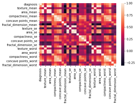
Next, we compare the correlation between features and remove one of two features that have a correlation higher than 0.9
columns = np.full((corr.shape[0],), True, dtype=bool)
for i in range(corr.shape[0]):
    for j in range(i+1, corr.shape[0]):
        if corr.iloc[i,j] >= 0.9:
            if columns[j]:
                columns[j] = False
selected_columns = data.columns[columns]data = data[selected_columns]Now, the dataset has only those columns with correlation less than 0.9
Selecting columns based on p-value
Next we will be selecting the columns based on how they affect the p-value. We are the removing the column diagnosis because it is the column we are trying to predict
selected_columns = selected_columns[1:].valuesimport statsmodels.formula.api as sm
def backwardElimination(x, Y, sl, columns):
numVars = len(x[0])
for i in range(0, numVars):
regressor_OLS = sm.OLS(Y, x).fit()
maxVar = max(regressor_OLS.pvalues).astype(float)
if maxVar > sl:
for j in range(0, numVars - i):
if (regressor_OLS.pvalues[j].astype(float) == maxVar):
x = np.delete(x, j, 1)
columns = np.delete(columns, j)
regressor_OLS.summary()
return x, columnsSL = 0.05
data_modeled, selected_columns = backwardElimination(data.iloc[:,1:].values, data.iloc[:,0].values, SL, selected_columns)This is what we are doing in the above code block:
We assume to null hypothesis to be “The selected combination of dependent variables do not have any effect on the independent variable”.
Then we build a small regression model and calculate the p values.
If the p values is higher than the threshold, we discard that combination of features.
Next, we move the result to a new Dataframe.
result = pd.DataFrame()
result['diagnosis'] = data.iloc[:,0]
Creating a Dataframe with the columns selected using the p-value and correlation
data = pd.DataFrame(data = data_modeled, columns = selected_columns)Visualizing the selected features
Plotting the data to visualize their distribution
fig = plt.figure(figsize = (20, 25))
j = 0
for i in data.columns:
    plt.subplot(6, 4, j+1)
    j += 1
    sns.distplot(data[i][result['diagnosis']==0], color='g', label = 'benign')
    sns.distplot(data[i][result['diagnosis']==1], color='r', label = 'malignant')
    plt.legend(loc='best')
fig.suptitle('Breast Cance Data Analysis')
fig.tight_layout()
fig.subplots_adjust(top=0.95)
plt.show()
Now we split the data to train and test set. 20% of the data is used to create the test data and 80% to create the train data
x_train, x_test, y_train, y_test = train_test_split(data.values, result.values, test_size = 0.2)Building a model with the selected features
We are using a Support Vector Classifier with a Gaussian Kernel to make the predictions. We will train the model on our train data and calculate the accuracy of the model using the test data
svc=SVC() # The default kernel used by SVC is the gaussian kernel
svc.fit(x_train, y_train)
Making the predictions and calculating the accuracy
prediction = svc.predict(x_test)We are using a confusion matrix here
cm = confusion_matrix(y_test, prediction)
sum = 0
for i in range(cm.shape[0]):
    sum += cm[i][i]

accuracy = sum/x_test.shape[0]
print(accuracy)
The accuracy obtained was 0.9298245614035088
Building a model without feature selection and comparing the results
Next, we repeat all the above steps except feature selection, which are:
Loading the data
Removing the unwanted columns
Encoding the categorical variable
Splitting the data into train and test set
Fitting the data to the model
Making the predictions and calculating the accuracy
data = pd.read_csv('../input/data.csv')
result = pd.DataFrame()
result['diagnosis'] = data.iloc[:,1]
data = data.iloc[:,2:-1]
label_encoder = LabelEncoder()
data.iloc[:,0] = label_encoder.fit_transform(data.iloc[:,0]).astype('float64')
x_train, x_test, y_train, y_test = train_test_split(data.values, result.values, test_size = 0.2)
svc = SVC()
svc.fit(x_train, y_train)
prediction = svc.predict(x_test)
cm = confusion_matrix(y_test, prediction)
sum = 0
for i in range(cm.shape[0]):
    sum += cm[i][i]

accuracy = sum/x_test.shape[0]
print(accuracy)
The accuracy obtained was 0.7017543859649122
Here we can see that the accuracy of the predictions is better when proper feature selection is performed
Click here to get this article as a IPython Notebook
Sir, I am getting strange result. Just copying/pasting your codes in my PyCharm IDE and using the same cancer data (downloaded from the website), I get lower accuracy with feature selection compared to without feature selection.